Amazon Redshift tutorial: Amazon Redshift is a cloud data warehousing tool that is available in AWS and it is the fastest cloud data warehousing tool available. Companies like SoundCloud and Philips or few among the thousands of companies who use Redshift for their data warehousing needs.
It is very easy to get started with redshift and also guys after reading this series of articles for Amazon Redshift tutorial, you will be able to start with Redshift independently.
AWS Redshift tutorial: Introduction to Amazon Redshift
Amazon Redshift is a fully managed petabyte-scale data warehouse service in the cloud. You can scale this particular service up to petabytes.
You can start with just a few hundred gigabytes of data and scale to a petabyte or more this enables you to use your data to acquire new insights for your business and customers so it provides you so much of storage you can store a lot of data and also it has a different kind of architecture.
Amazon Redshift manages all the work of setting up, operating and scaling a data warehouse. It takes care of everything because that’s what AWS does for us and these tasks include provisioning capacity monitoring. You know if we get metrics for almost every service then backing up the cluster we can backup using snapshots automated and applying patches and upgrades to the Amazon redshift engine.
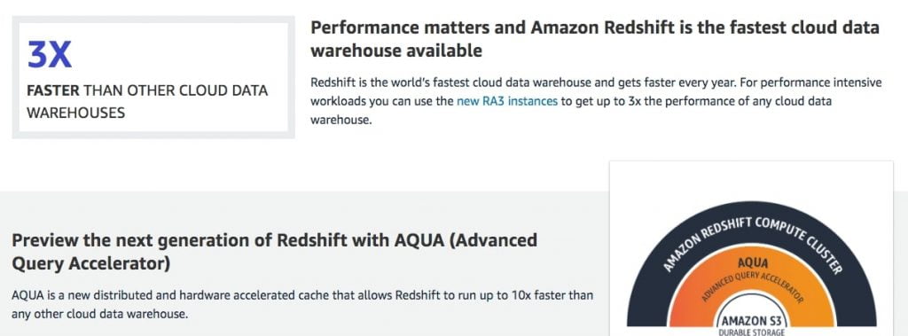
AWS gives us the confidence that Redshift is three times faster than the other data house is available. Amazon Redshift is the world’s fastest cloud data warehouse and gets faster every year for performance-intensive workloads you can use.
The new RA 3 instances to get up to 3x or the performance of any data cloud data. You need to choose the size of your redshift cluster based on the performance requirements and only pay for the storage that you use. The new managed storage automatically scales your data warehouse storage capacity without you having to add and pay for additional compute instances.
Redshift automatically scales a data warehouse storage capacity for us yeah so this is automatically done we don’t need to provision or we don’t need to do anything.
AWS Redshift makes it simple and cost-effective to run high performing queries on petabytes of structured data so that you can build powerful reports and dashboards using your existing BI tools and you can get insights out of it and operational analytics on business events bring together structured data from your data warehouse and semi-structured data such as application logs from your s3 datalink to get real-time operational insights on your applications and systems.
Amazon uses redshift and it’s working well for them and then coming to McDonald’s Amazon redshift enables faster business insights and growth and provides an easy to manage the infrastructure to support our data workloads redshift has given us.
What is Redshift?
It is a data warehousing tool provided by Amazon and you can use it for analytics and you can use it for getting operational insights and you can use it as the data provider for your BI tool.
AWS Redshift tutorial: Concepts of Amazon Redshift
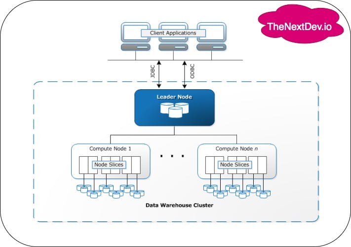
This is the data warehouse architecture of AWS Redshift so they have a leader node and they have multiple computers. You can have multiple compute nodes and all those compute nodes have node slices.
They provide you two different connectivities
- JDBC
- Java Connectivity
- ODBC
- open connectivity
you can use them to connect with your client applications.
Client:
Redshift structure is built on a PostgreSQL database so most existing SQL client applications will work with only minimal changes. So you can use this with your MySQL workbench or SQLserver or other clients. You can also use the PostgreSQL client.
AmazonRedshift communicates with client applications by using industry-standard JDBC and ODBC drivers. You can use either of them
Clusters:
- The leader node executes the code for individual elements of the execution plan and assigns the code to individual compute nodes.
- For example, if a huge query comes in so the leader node takes it. It splits up the query into smaller queries or smaller tasks it provides it to the available compute nodes respectively
- The leader node decides how to distribute the load
- You don’t need to pay anything for the leader node you just pay for the number of compute nodes you create and yeah a cluster is composed of one or more compute nodes
- The cluster can have one or more compute nodes and if a cluster is provisioned with two or more compute nodes an additional leader node coordinates the compute nodes and handles external communication
- For example, if you have only one compute node if you create it with just one compute node there is no need of a leader node to distribute work among the other compute nodes because there is only one node and all the work will be assigned to that so there is no use of leader node
- so what if you assign more than two or two compute nodes then a leader node is automatically assigned and all the incoming queries all the incoming transactions are taken care
- leader node takes care of it divides into multiple smaller tasks and provided to the compute nodes accordingly and your client application interacts directly one with leader node the compute nodes are transparent to the external applications
- client applications do not contact the compute nodes available if you have two or more nodes two or more compute nodes then your client applications only point of connectivity is the leader node, not the compute nodes
- all the requests first go to the leader node then it goes to the compute node
- The leader node manages communications with client programs in all communication with compute nodes. It takes care of all the communication between the client programs and the compute nodes it stands in the middle it’s like a middleman and it parses and develops execution plans to carry out database operations
- Any kind of a huge database operation will be taken care of at the leader node. The leader node will assign the work to the compute nodes accordingly.
If you hit in a complex query it first goes to the leader node here it is the first point of contact for any clients applications the leader node now splits it up accordingly it splits it up in multiple parts and provides it to other compute nodes which do their part and provide the results back.
The leader node aggregates them into a single result and sends it back to the client application so this is why we need a leader node based on the execution plan.
Each compute node has its own dedicated CPU memory attached disk storage.
Amazon Redshift provides two node types: dense storage nodes and dense compute no. The dense compute notes will have a lot of computing power and the dense storage nodes are used for scaling up your storage whenever you need for scaling down
Each compute node is partitioned into slices and each slice is allocated a part of the node’s memory and disk space where it processes a portion of the workload assigned to the node.
AWS Redshift tutorial: Amazon Redshift performance
The performance of AWS Redshift, there are six factors that to be available in redshift which makes Redshift’s performance faster
- Massively parallel processing
- Columnar data storage
- Data compression
- Query optimizer
- Result caching
- Compiled code
Massively parallel processing
Multiple compute nodes manage all database query processing leading up to a result aggregation within which each core of every node executing identical compiled database query segments on portions of the complete data. So this is the core function of massively parallel processing. It works the same as a leader node functions.
Basically massively parallel processing enables fast execution of complex queries on large amounts of data. The leader node splits up the workload, provides it to multiple compute nodes. The processing is happening parallelly. In the last, all of the results are coupled up together and then provided
Columnar storage
In a traditional database, the database blocks size ranges from 2 KB to 32 KB. Amazon Redshift, the block size can go up to 1 MB which is more efficient and further reduces the number of input-output requests needed to perform any database loading or any other operations which are part of database query execution.
In Redshift, any data coming in will be automatically taken into columnar storage. In redshift data of this entire column stored one block so basically if there are six columns then there will just be six blocks of which have all the column data.
Columnar storage provides better performance. The columnar storage type for database tables is that the most vital factor in optimizing analytic query performance because it drastically reduces the general input-output requirements and reduces the quantity of information you would like to load.
In row-based storage, in each row, there will be one block so this will basically not take up a lot of storage but it will take a lot of memory.
A data warehousing tool is used for analytics on large amounts of data, so let’s say you want to calculate the average age from 100,000 records of age so if you try to analyze through row-based storage it will go into every block and gather that particular data and then it will do the process.
But in the case of columnar storage, it just takes this block so there will be one single block and it just uses that this reduces the input requirements, and also it increases their performance.
Because of columnar storage, Amazon Redshift tells it is three times faster than using a row-based.
Data compression
Data compression reduces storage requirements thereby reducing disk input/output which improves query performance. If you compress the data it will reduce storage requirements so when you exceed a query the compressed data is read into memory then uncompressed during query execution
Loading fewer data into memory enables Amazon Redshift to allocate more memory to analyzing the data.
Data compression is started automatically in Redshift, no additional setting required.
Query optimizer
The Amazon Redshift query execution engine incorporates a query optimizer that is massively parallel processing aware and takes advantage of the columnar oriented data storage
There is a separate query optimizer inside redshift which is running for us and it reduces query execution time which improves system performance.
Result caching
Amazon Redshift caches the results of certain kinds of database queries in memory on the leader node. For example, multiple people are attempting to execute the same database query. For analysis, these people are querying to the same Redshift cluster again and again.
In this case query data automatically gets stored in the cache of the leader node, so data retrieved faster than going back to the compute nodes then querying it back before providing the final result.
It also does a result caching so when a user submits a query Amazon Redshift checks the result cache for the valid or cached copy of the query result if a match is found in the result cache.
Amazon Redshift uses the cached resource and does not execute the query so when you run that query once again query execution does not happen so this improves the performance because it just takes the results from the cache and gives it back.
This results in faster execution speed especially for complex queries
All these performance features are already implemented in the Redshift there is no need to trigger
AWS Redshift tutorial: Amazon Redshift workload management
Workload management (WLM) allows users to flexibly manage priorities within workloads so that short fast-running queries won’t get stuck in queues behind long-running queries.
Amazon Redshift workload management (WLM) creates query queues at runtime in line with service classes, which define the configuration parameters for various kinds of queues, including internal system queues and user-accessible queues. Fa A user-accessible service class and a queue are functionally equivalent.
When you run a database query, WLM assigns the query to a queue consistent with the user’s user group or by matching a database query group that’s listed within the queue configuration with a question group label that the user sets at runtime.
With manual workload management (WLM), Amazon Redshift configures one queue with a concurrency level of 5, which enables up to 5 queries to run concurrently, plus one predefined Superuser queue, with a concurrency level of 1. you’ll define up to eight queues. Each queue is often configured with a maximum concurrency level of fifty. The utmost total concurrency level for all user-defined queues (not including the Superuser queue) is 50.
The easiest thanks to modifying the WLM configuration is by using the Amazon Redshift Management Console. you’ll also use the Amazon Redshift command-line interface (CLI) or the Amazon Redshift API.
If you are reading Amazon Redshift Tutorial first time and new to cloud computing then you should first understand the basics of cloud computing
Reference has taken from Amazon Redshift developer guide


